Simulating a stringed instrument

This was a fun project I initially undertook in October 2023. I was curious to see how vibrating strings looked under conditions actually found in musical instruments, and then took off in various directions, exploring frequency distributions of different picking locations and trying to generate audio from the simulations. You can find all the code for this at the GitHub repository: github.com/ELFREELAND/string_instrument

What is this?

When you watch someone play a guitar, it’s hard to make out exactly how the strings are vibrating – all you can really see is a blur. If we want to see what the strings are doing on the scale of milliseconds, we would need a really expensive camera. Alternatively, we can simulate the strings using some simple physics, and get a pretty good idea of what the strings are probably up to.

The Classical Wave Equation

Waves in a string are traditionally represented by the wave equation, a 2nd-order linear partial differential equation (PDE)¹:

$\frac{\partial^2u}{\partial t^2}=c^2\frac{\partial^2u}{\partial x^2}$

$u(x,t)$ represents the displacement of the string at position $x$ , time $t$ . The left side of the equation represents the acceleration of the string, and the right side is related to the curvature of the string. You should read this as: “the acceleration of a point on the string is proportional to the curvature of the string at that point”. The constant $c$ is the propagation speed of a wave in the string, and it is equal to the square root of the tension divided by the linear density of the string:

$c=\sqrt{\frac{T}{\rho}}$

This equation can be solved without too much trouble. For a string that is fixed at both ends, the boundary conditions are stated $u(0,t)=u(L,t)=0$ , and solutions are of the form:

$u(x,t)=A\sin\left(\frac{n\pi x}{L}\right)\sin\left(\omega t\right)$

$n=1, 2, 3\dots$

The fact that this is a linear PDE means that any two solutions can be added to get a third solution. The important takeaway from this is that any solution of the wave equation can be expressed as a sum of sine-wave-like solutions. Each possible value of $n$ is called a harmonic.

If we introduce damping into the system, the classic wave equation becomes:

$\frac{\partial^2u}{\partial t^2}=c^2\frac{\partial^2u}{\partial x^2}-\mu(x)\frac{\partial u}{\partial t}$

where $\mu$ represents the strength of damping. You should read this as “the acceleration of the string is proportional to the curvature of the string, minus some friction which varies with how fast the string is vibrating”. The variation of $\mu$ with $x$ is important, since selectively damping the strings allows the musician to vary the tone of the instrument.

The System

We’re going to model the E string on my bass guitar, which looks like this:

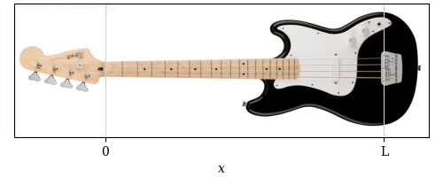
The origin of the x-axis is at the nut, where the strings enter the neck. The string ends at the bridge, where $x=L$ .

The oval-shaped protrusion to the left of the bridge is the pickup, an device which uses electromagnetic induction to convert the vibration of the strings into an electrical signal. We will get an “electrical signal” from our simulation by sampling the displacement of the string at a single point.

The fundamental frequency of a vibrating string, $f_0$ , is related to the wavelength $\frac{1}{L}$ and the wave speed $c$ by:

$f_0=\frac{c}{2L}=\frac{\sqrt{T}}{2L\sqrt{\rho}}$

this is known as Mersenne’s law. The fundamental frequency of my bass’s E string is 41.2 Hz, the string is 30 inches or 0.762 m long, and the manufacturer quotes the tension at 29.6 pounds or 131.67 Newtons, which gives a linear density of 0.033 kg/m.

The Initial Condition

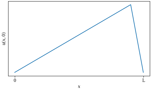
There are a number of ways to set a string in motion. The simplest of these involve pulling on the string at a single point and releasing it, meaning the initial condition of the freely-vibrating string looks like a triangle:

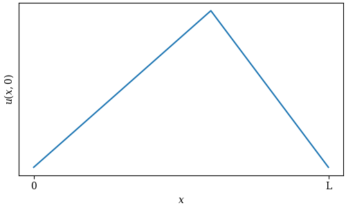
We can choose to pluck the string close to the bridge or closer to the middle, which will affect the timbre of the instrument:

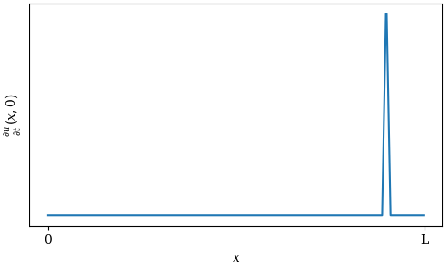
Alternatively, instead of pulling and releasing the string, we can quickly strike it. This is a common technique among bass players, both upright and electric; and it’s also the mechanism behind the sound of a piano. This condition can be modeled by zero initial displacement, but a local spike in initial velocity:

Damping

The effect of damping on the string’s behavior is one of the more interesting things to investigate here. We’ll look at two important cases: palm muting and harmonics.

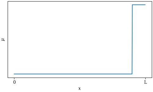
Palm muting is an important guitar technique, especially in rock and metal music, which involves the guitarist holding the side of their picking hand against the strings near the bridge to mute them. This can be approximated by a higher value of $\mu$ right next to the bridge:

Playing harmonics is a technique used for any number of string instruments. By lightly muting the string at position $\frac{L}{n}$ , every harmonic will be muted except those that have a node³ at that position. For example, my muting the string at position $\frac{L}{2}$ :

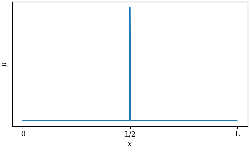
we can isolate even-numbered harmonics. By muting at $\frac{L}{3}$ :

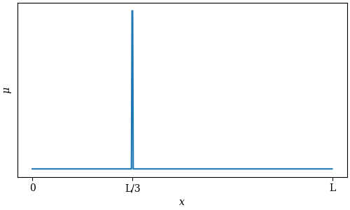
we can isolate harmonics that are multiples of 3.

The Numerical Approach

Since we are dealing with complicated damping conditions, we are going to outsource all the thinking to a computer. In order for the computer to simulate the string, we’ll need to discretize it.

Instead of a continuous string of constant linear density $\rho$ , let’s consider a massless string loaded with uniformly spaced point masses of mass $m$ spaced distance $\Delta x$ apart, such that $\frac{m}{\Delta x}=\rho$ . The acceleration of each particle depends on how far it is from each of its neighbors, which gives a discrete version of the second derivative. For particle $i$ :

$\frac{d^2u_i}{dt^2}=c^2\frac{u_{i+1}+u_{i-1}-2u_i}{\Delta x^2}-\mu_i\frac{du_i}{dt}$

If particle $i$ is exactly halfway between its neighbors, it will experience zero acceleration (save for that caused by damping). If its displacement is greater or less than the average of its neighbors, it will experience an acceleration towards their average. The particle will also experience an acceleration proportional to the magnitude of its velocity and opposite its direction, due to damping.

We have replaced our single 2nd-order PDE with a system of 2nd-order ordinary differential equations (ODEs)². However, the solver we’ll be using only operates on 1st-order equations. To proceed further, we’ll need to turn our system of 2nd-order ODEs into twice as many 1st-order ODEs.

We can do this with the following substitution:

$v_i=\frac{du_i}{dt}$

$\frac{dv_i}{dt}=\frac{T}{\rho}\frac{u_{i+1}+u_{i-1}-2u_i}{\Delta x^2}-\mu_i v_i$

For every point on the string, we will have one copy of each of the above equations. I have chosen to use 500 points, meaning the solver will have to chew through 1000 first-order ODEs. Take a look at the GitHub if you want to see how exactly I make this happen.

Results

Waveforms

First, what do the waveforms look like? The figure below shows the displacement of the string at 75% of its length for one second after it’s plucked – this is like assuming the pickup is located at 75% of the length of the string. In order, they are an open string plucked near the bridge, an open string plucked near the neck, an open string hammered, a palm-muted string plucked near the bridge, a string muted to produce the 2nd harmonic, and a string muted to produce the 3rd harmonic.

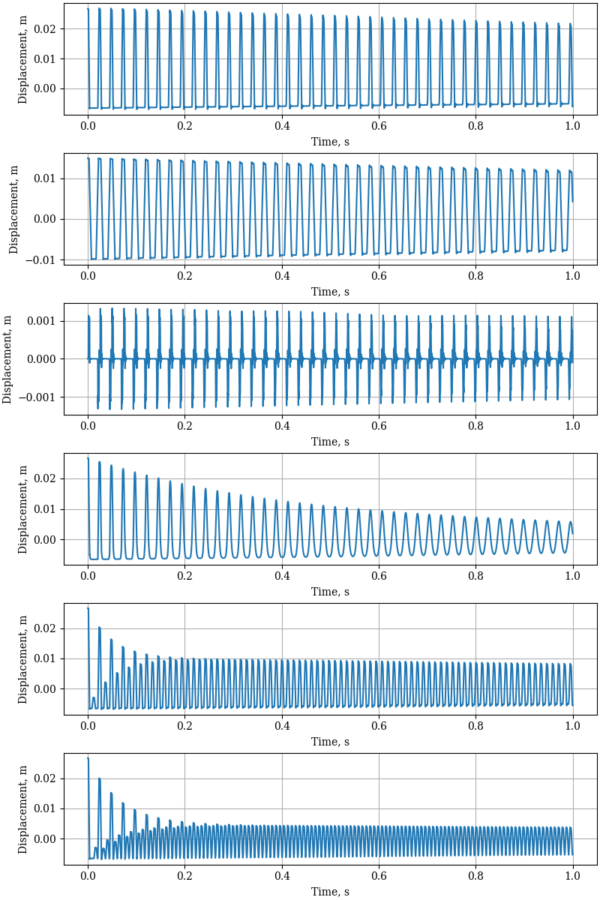
We can see that the muted strings take some time to reach their final states – the palm-muted string’s waveform decays in amplitude and becomes smoother, while the harmonic-muted strings take some time to develop the higher frequency components.

Let’s look a little closer at the waveforms, halfway through the simulation:

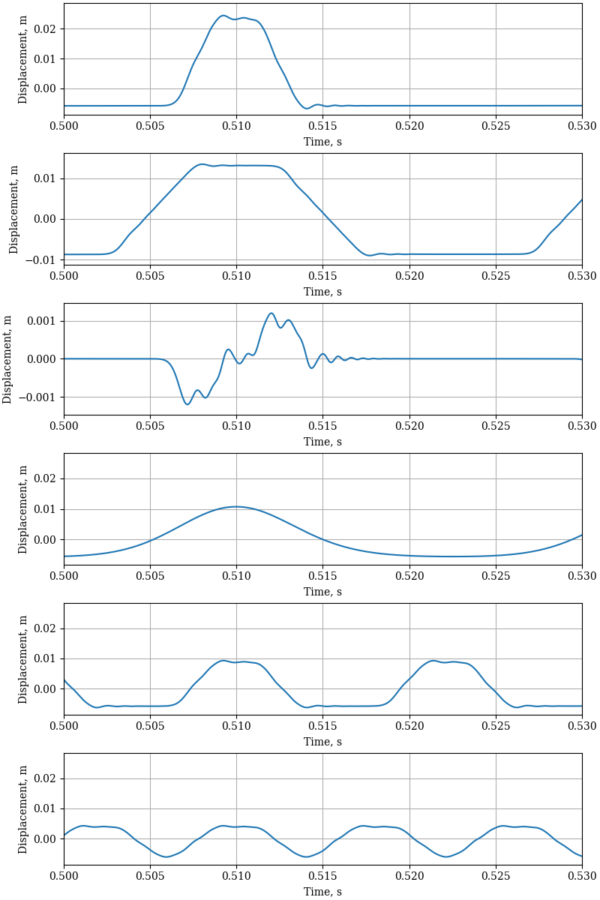
The plucked open strings have a sort of plateau-shaped waveform, the hammered string has a sort of jittery pulse shape, the palm muted string has a very smooth shape reminiscent of the string plucked near the neck, and the harmonic-muted strings have plateau-like waveforms at a higher frequency than the open strings.

Frequency spectra

Remember how any solution of the wave equation can be represented as a sum of sine waves? We can exploit a similar identity in the waveforms at the pickup using a tool called a Fourier transform (four-ee-ay). We can apply a Fourier transform to the waveform data, and get back a data set like this:

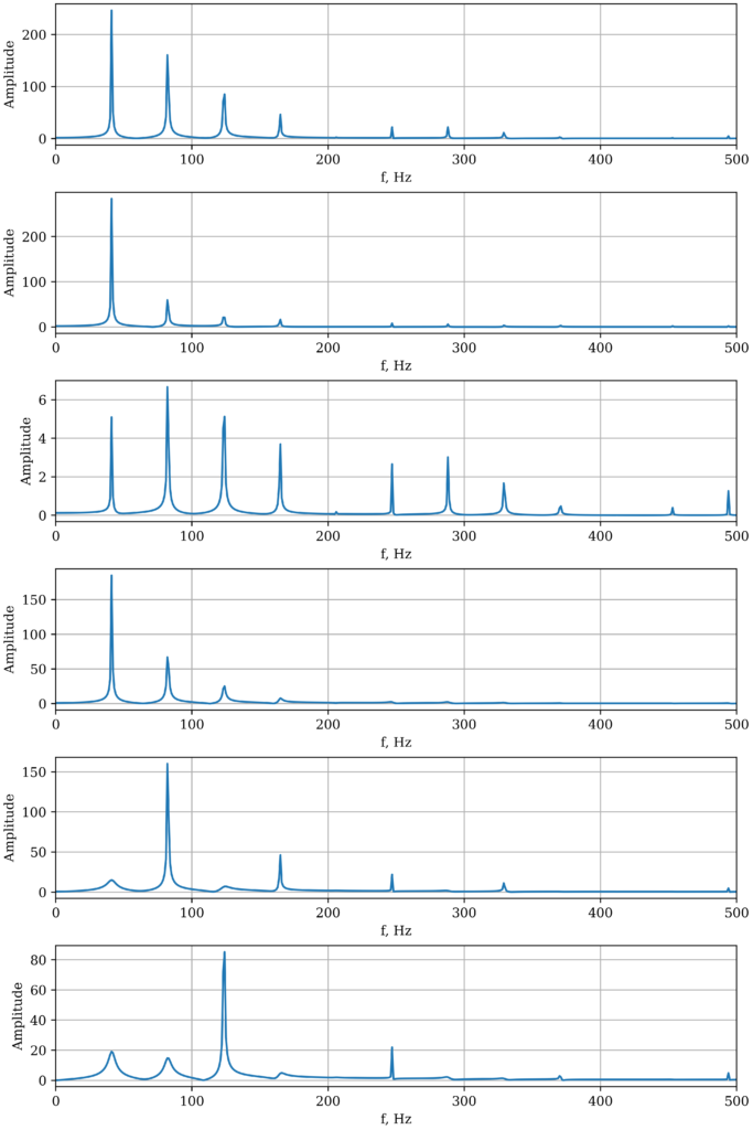
The spikes at certain frequencies tell you that a sine wave at that frequency comprises a large part of the waveform. The first two spectra have large spikes at about 40 Hz – that’s the fundamental. The first spectrum – plucked near the bridge – has larger amplitudes of the 2nd, 3rd, and 4th harmonics than the spectrum plucked near the neck. Plucking near the bridge is generally known to produce a “brighter”, “clankier” sound on a guitar or bass, and this corresponds to a higher amplitude of higher harmonics.

The spectrum of the hammered string is interesting – the fundamental is not the component with the highest amplitude; instead it is the 2nd harmonic. The 3rd, 4th, 6th, 7th, and 8th harmonics also have a substantial amplitude. As you’ll see later, the hammered string has a very interesting sound, likely influenced by this diverse frequency spectrum.

The palm-muted string has very low amplitudes of everything above the 4th harmonic – all higher harmonics have been silenced by the musician’s hand. This is kind of the point – palm muting gives a more subdued sound, allowing the instrument to sit lower in the ensemble.

Remember what is happening in the harmonic-muted strings: every harmonic that isn’t a multiple of 2 or 3 is muted. This is clearly visible in each spectrum – in the 2nd-harmonic-muted string, there are spikes at about 82, 164, 246, and 328 Hz, corresponding to even harmonics. In the 3rd-harmonic-muted string, there are spikes around 123, 246, 370, and 492 Hz, which are harmonics that are multiples of 3. Note that there are still small spikes at the fundamental and the first couple harmonics, since these are present in the first few vibrations of the string.

Finally, note that in every spectrum, the 5th harmonic, around 205 Hz, is absent or very nearly so. The 5th harmonic has nodes at 25%, 50%, and 75% of the string’s length. This happens to line up with where the pickup is sampling the string’s vibration, so the 5th harmonic is not detected. The 5th harmonic may well be present in the string’s vibration, but it doesn’t contribute to the signal we get.

Animation

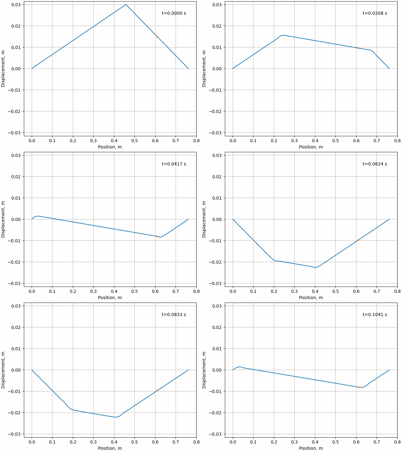
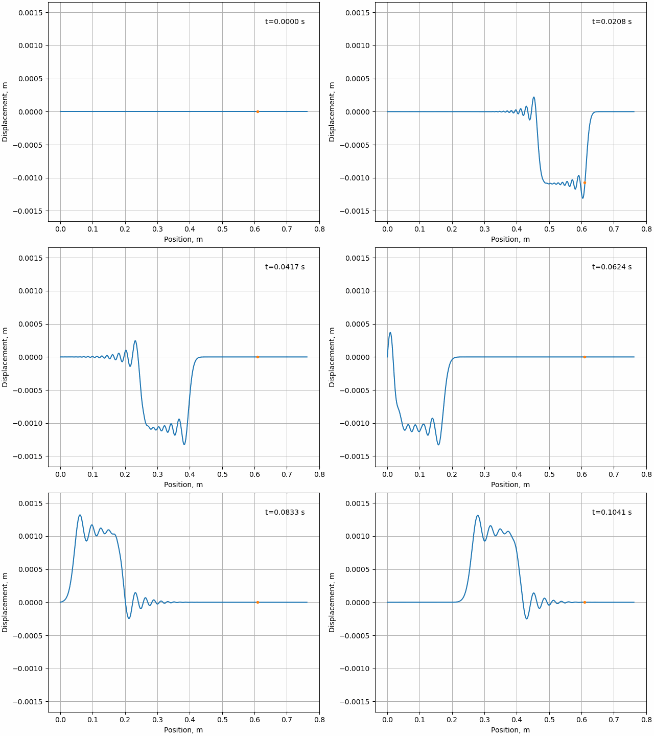
But what does the string actually look like? We can use matplotlib.animation to create videos of the string in motion. I’ve highlighted the point where we sampled the displacement (the pickup) with a dot.

Open string, picked near the bridge:

Open string, picked near the neck:

Open string, struck:

Palm-muted string:

String muted to produce 2nd harmonic:

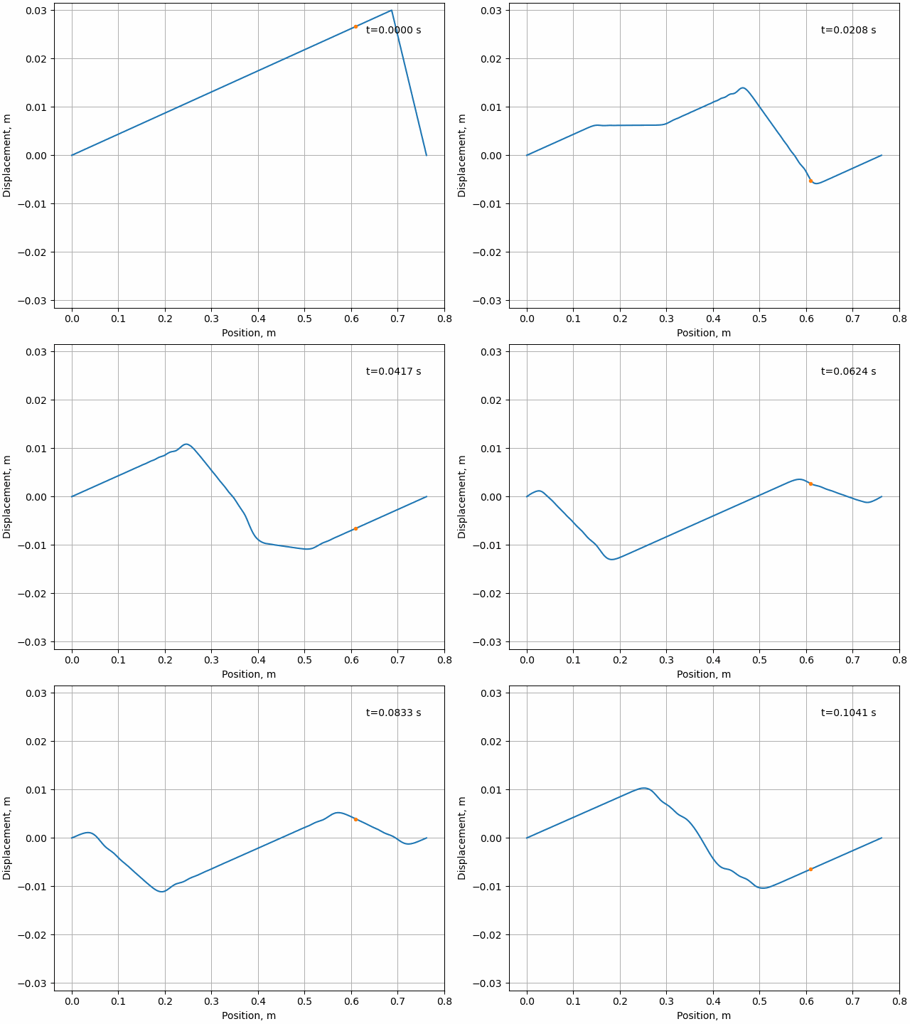
String muted to produce 3rd harmonic:

I think the harmonic-muted strings are the most interesting here. You can see the initial wave reflect off of the muted point, then off the end of the string, and interfere with itself to produce the higher harmonics. Visualizing harmonics was actually the initial reason I started this project, so this was really cool to see.

Audio

Finally, we can use python’s built in wave library to output the displacement data to .wav files. The audio below contains all 6 waveforms (in the same order as before) played at a pitch of E1, then at a pitch of E4 (329 Hz), then a bassline from a song I like, created from the hammered open string and palm muted string sounds.

You can hear how the open string plucked near the bridge sounds “brighter” than the same string plucked near the neck, and the hammered string sounds “buzzy” or “clanky”. The palm muted string fades away quickly, giving a more subdued sound, and the harmonic-muted strings sound an octave higher and an octave plus a fifth higher than the others, respectively. When the harmonic-muted strings are played at E1, you can also hear how they take a few fractions of a second to develop the higher harmonics fully.

What else?

I still have a few questions that I didn’t end up getting to.

Can we use less than 500 points in the string and get similar results? like, can we use 50? 10?

The wave equation is accurate when the curvature of the string is small compared to its width. If the string is wide or the curvature is large, the proportionality in the wave equation starts to fall apart because the bending moment of the string starts to contribute to the vibration, in addition to the tension. Can we model that?

Notes

¹An equation that expresses rates of change of a quantity (string displacement) in terms of rates of change of several other quantities (time, and position on the string). Second-order means it’s actually talking about the rate of change of the rate of change.

²An equation that expresses rates of change of a quantity (string displacement), in terms of rates of change of one other quantity (time).

³A point where the sine wave is at zero.